
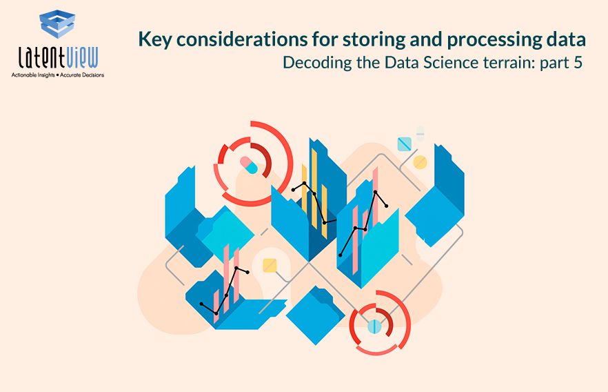
Decoding the Data Science Terrain: Part 5
In the four previous posts in this series, we talked about a framework for mapping the data science terrain (part 1), discussed ways to monetize and extract value from information (use cases, part 2), look at where datasets reside (part 3), and how data is extracted from sources (part 4).
In this post, we will describe the key considerations for storing and processing data in the context of analytic needs of the users.
Within a given enterprise, the analytical capabilities and needs of the audience are quite varying, such as: regular reporting, ad-hoc analytics, data services, iterative models, real-time transformations, etc. Creating the architecture to maintain consistency of data, while meeting every type of end user analytics need, is a fundamental challenge when developing a modern data landscape.
Storage
In this section, we will consider three aspects of data storage that impact scalability and performance of the solution: choice of data model (Relational vs Non-relational), data model design (OLAP vs OLTP) and storage engine (Columnar vs Row-based approaches).
Data Model Types: Relational vs Non-Relational
There are many types of data models, including Relational, OLAP, Graph, Document, etc. Let’s briefly look at the pros and cons of each, from an analytics perspective.
Relational Model
While relational model was invented for run-of-the-mill business processing, they have scaled well and have been effectively adopted for analytics use cases. Relational model works very well for a wide range of use cases because it defines a declarative approach (SQL) to working with the data. This means the user just tells the system the shape of the results required (the filters, the aggregates, the joins, etc.), and lets the engine figure out how to deliver the results. This is in contrast to an imperative approach, where the user not only has to decide what he needs, but also how to get it done.
The fundamental assumption of a relational model is that all data is represented as mathematical relations (expressed as Tables), each of them consisting of a heading and a body. A heading is a set of attributes and a body is a set of tuples (rows in the Table).
Non-Relational Models
The most prominent alternatives to a relational model for big data are documents and graphs. The first one is not suitable for analytics, since they do not allow for joins or for many-many relationships.
However, graph data model excels in certain types of analytics use cases, such as identifying degrees of separation between two nodes in a network. It could be people in a social network, entities in a corporate network, or actors in a movie database. As the number of many-many relationships increase with corresponding increase in query, graph databases tend to perform much better than relational databases.
In a graph database, data is stored using nodes (e.g. actors, movies) and edges (e.g. actors in a movie). Just like SQL in a relational database, graph databases provide interfaces for users to query data using a declarative approach.
Data Model Design: OLAP vs OLTP
Within the relational model, data can be stored for transaction processing (On line transaction processing or OLTP) or for analytics (On line analytical processing or OLAP). For OLTP, data models are normalized to reduce redundancy and improve integrity.
However, for analysis purposes, data is stored in a de-normalized form for faster querying and promoting ease of use. There are many types of de-normalized storage, and we consider the most popular approach: Star Schema.
Star Schema
In a star-schema based de-normalized form, data is stored into a set of “fact” tables and “dimension” tables.
Fact tables capture transactions (e.g. every sale), periodic snapshots (e.g. inventory at end of day) or accumulating snapshots (item’s movement from entry to exit within a warehouse), and typically store numeric measures. These consist of many numeric measures as well as foreign keys to one or more dimension tables. Fact tables are both large and sparse, and they typically run into billions or even trillions of rows.
Dimension tables are used to store attributes of entities such as product, promotions, geography, time, etc. that are used to slice and dice the facts. Each dimension table contains numerous attributes (think of product attributes, such as price, category, brand hierarchy, Unit of Measure, batch number, manufacturer / vendor attributes, etc.). Dimension tables are typically much smaller than fact tables and the largest ones may run into tens of millions of rows (think of customer dimension for a large retailer).
For example, the following picture provides an overview of a star schema model for capturing sales in a store, by product and date. Note that the grain of the data in the picture above is one row per product per store per day, i.e. it does not capture every sales transaction, but captures a snapshot of daily sales by product for every store.
There are many nuances to designing and delivering facts and dimensions, and this is a vast area of specialization. For those who are interested, please take a look at the following excellent books by Ralph Kimball, et al: The Data Warehouse Toolkit and The Data Warehouse ETL Toolkit.
ROLAP vs MOLAP
Multi-dimensional databases are a specialized class of data stores that package “data cubes” of metrics and dimensions. These cubes can be powered using relational databases or through specialized databases called Multi-dimensional databases. When the star schema leverages a relational model, the resulting OLAP is called ROLAP. When it leverages a multi-dimensional database such as Cognos TM1 or Essbase, the resulting OLAP is called MOLAP.
While ROLAP tools are very good when it comes to scaling the performance on high-cardinality datasets, they come with the added complexity of requiring additional steps in the ETL process to load the aggregates.
Storage Engine: Row-oriented vs Columnar
What if the fact table has billions or trillions of rows? How do we optimize this for querying? When a user runs a query, several blocks of data are moved from disk to memory. Once it’s moved into memory, the processing is very quick. The fundamental bottleneck in querying arises from moving data from disk to memory (i.e., the Input / Output or I/O).
In MPP databases that power the big data world, data is spread across multiple nodes or partitions, each with its own CPU and disk. When a user performs a query, each partition fetches data from its disk, moves it into memory and then does the computation before returning the results.
Let’s consider a fact table that has a billion rows, such as sales_transaction_fact spread across 20 nodes, with each row containing 50 columns. The graphic below describes how this works.
In the graph above, each block of data contains all the columns in a given row. Since data is moved in blocks, data in all the columns are read into memory irrespective of whether they are used in the query or not. This is a waste of I/O capacity, and it is unnecessary, because typical user queries contain only a small subset of columns.
In a columnar database, every data block holds a single column. This provides a significant lift in performance over row-oriented data stores, because only those columns that are needed for the query are read from the disk through I/O. This leads to significant reduction in latency compared to row-oriented approaches.
In addition, each block can achieve higher compression ratios in columnar format. This is because the data in a column is more homogenous compared to the data in a row. This further reduces the time spent on I/O.
In a typical columnar database, there exists a leader node, which manages the distribution of data and builds the plan for slave (compute) nodes to follow. This works really well and scales linearly when the data is spread evenly across nodes. In other words, if the data is spread evenly, doubling the number of nodes will double the throughput.
However, we need to ensure that the keys are distributed evenly, and also take into account query patterns to decide how the data is distributed. For example, if there is a large fact table (sales fact) and a large dimension table (customer dimension) and a few small dimension tables (time dimension, geography dimension, etc.), it’s best to distribute both the fact and the large dimension by the customer_id key so that matching values from both of the large tables are co-located in each node. It’s also a good practice to copy the smaller dimensions to every node.
As you may have guessed, there are many nuances in data model design, such as distribution and sorting (which we haven’t seen here). This has significant potential to affect query performance, and hence it’s important to understand this in great detail before we design data models.
Data Processing
The second topic we’re going to discuss in this blog is processing. There are two broad approaches to processing data – batch processing and stream processing.
Batch Processing
For simple to moderately sophisticated environments, batch processing can be accomplished with a combination of various UNIX tools that are a series of small programs that act in consort, in the form of a pipeline. The advantage of these tools is that they are simple to develop and maintain, for moderately complex environments.
However, these tools do not support sharing and reuse of business rules across multiple pipelines, managed loading of data, multi-threaded operations, and so on. If we need these capabilities, it’s best to look at more sophisticated ETL tools such as traditional ETL tools like Informatica, modern data preparation tools like Alteryx or big data tools like those in the Hadoop ecosystem.
Regardless of whatever the environment is, batch processing involves the following sequence of steps:
Of course, this is a simplistic picture. There are numerous complexities in a typical real-world data environment that needs to be handled, such as, slowly changing dimensions, multi-valued dimensions and bridge tables, ragged hierarchies, late arriving dimensions, generating surrogate keys for dimensions, multiple units of measures, late arriving facts, aggregating fact tables, etc.
Stream Processing
There are three main considerations when designing a stream-based architecture: where they originate, how they are delivered to consumers, and how they are processed. Let’s look briefly at each of these.
Where do Streams originate?
Life doesn’t happen in batches, but in streams. In a streaming world, the input data is delivered as a continuously flowing, time-stamped, immutable event objects. The sources of streams could be IoT devices sending status messages at periodic intervals, mobile devices transmitting state, electronic meters sending energy consumption data periodically, and numerous other examples.
Streams can also arise from mundane business applications or even from databases. For instance, the database logs of OLTP databases can emit every update to the data in the form of a stream of events. It’s possible to capture these changes and process them, rather than do it in batch mode, as is currently done today in most cases.
How do Streams get delivered to consumers?
Events are generated by producers, but they are typically not transmitted to consumers directly. This is because, there may be multiple consumers that may want to consume data at their own pace, and there may be requirements for robust failure handling. Hence, a message broker is a typical pattern that is used to mediate between producers and consumers.
Today’s message broker landscape is dominated by open source tools such as Kafka, ActiveMQ, RabbitMQ, etc.
Some of the primary considerations in developing a broker-based solution are the following:
- What happens when producers generate messages faster than consumers can consume?
- What happens when there are many consumers that want to consume a given message?
- What happens when the processing requires that every message needs to be consumed exactly once, even when there are many consumers?
- How do we ensure that a consumer has successfully completed handling the message before it is removed from the broker?
- What if there is a need to store the messages so they can be re-processed by new consumers in the future?
- How can we ensure scalability of the architecture when the no. of messages produced becomes very high?
The answers to these questions determine the pattern of streaming architecture to use. Tools like Apache Kafka use a distributed log approach to store every message and then wait for consumers to consume them. They support multiple consumers through a pull model (i.e. the consumer is responsible for reading the message from the broker). They support robust handling against failures, arbitrary reprocessing of messages, etc.
Other set of brokers use a publish / subscribe model, wherein they provide transient message storage until the messages are processed by consumers. Once they are processed, the messages are deleted. To improve reliability, the broker can be set up to expect acknowledgment from consumers on successful handling of each message before they are deleted from the transient store. To ensure each message is processed exactly once, messages can be sent to exactly only one consumer at a time, or, to scale with increasing volume, messages can be transmitted (fanned out) to many customers at a time.
Stream Transformation
Stream transformation is an advanced topic of discussion and must be reserved for a future post. The key motivating questions are:
- How do we handle time in streaming systems? For example, in fraud detection systems, what happens if there’s a significant delay between the transaction time and validation time? How much window do you consider when looking at history?
- How do we correlate data in one stream to another stream? For example, how do we look at roll-out of a new feature in our web application and the resulting clickstream behavioral changes?
Hopefully, this post has provided a high level overview of various data storage and processing considerations for a modern enterprise.
Read part 1 of our blog series on ‘Decoding the Data Science terrain’ and learn more about the Data Science and Analytics framework. Click here to read part 2 of our blog series on ‘Decoding the Data Science terrain’! Find out how to evaluate the quality of data in part 3 of our blog series on ‘Decoding the Data Science terrain.’ Understand the steps in the data collection process in part 4 of this series.