Meta-Learning: An Overview and Applications

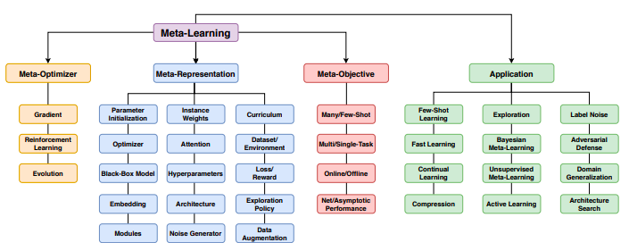
Introduction

Meta-Learning (Learning to Learn) is the science to design models that can learn new skills or adapt to various environments by observing how a learning algorithm performs learning and then learns from the metadata or learn to do new tasks much faster. 

Why do we need Meta Learning:

• Faster AI systems
• More adaptable to environment changes
• Generalizes to more tasks
• Optimize model architecture and hyper-parameters

The traditional way of machine learning research is by getting a huge dataset and then training a model from scratch on the data. This is very different from how we humans learn. They leverage their earlier learning to learn very quickly using a handful of data points. eg. Kids learn to differentiate between cats and dogs very quickly by seeing their pictures for just a few times.

Would it be possible to design a model that can learn fast and with fewer data samples? This is what Meta-Learning aims to solve.

The other differences between Meta Learning and traditional Machine Learning is on the scope of focus, for instance machine learning focuses on a certain task , for example breast cancer detection, where machine learning will focus on whether the the patient has a breast cancer or not; whereas the meta learning algorithm will focus on multiple tasks which will involve the traditional classification problem along with the best algorithm to predict and how to optimize the performance of the algorithm using hyperparameter tuning.

The areas of application of meta learning is huge and there are major research opportunities in the future.

Generic learning algorithm vs a Meta Learner

Learning Algorithm

• Input: Training data set Dtrain ={(xi,yi)} , where (xi,yi) is one data point. Let’s consider y as the dependent variable and x to be the independent variable
• Output: model M (the learner)  
• Objective: Good performance on test data set Dtest={(xi’,yi’)}, where the data points are unseen to the model

Meta-Learning Algorithm

• Input: A meta training set which contains a training set of datasets where each dataset is a split of the training set and its corresponding test sets. The training test set pair is often called episodes.

Dmeta-train= {(Dtrain,Dtest)}

• Output: parameters of an algorithm (meta-learner)
• Objective: Good performance on new episodes, new training-test splits for other problems

If the meta-learning algorithm does not give good results on unseen data sets, then it’s not really meta-learning. An ideal meta learner would be training and learning the procedure of hyperparameter optimization of a neural net , by training that on CIFAR-10 and showing that the algorithm also works on some other image classification problem. Although meta learning and transfer learning may sound similar sometimes, the high level difference would be Meta-learning is more about speeding up the learning process by learning to tune hyperparameters and are more general i.e can be used for multiple tasks whereas transfer learning uses a neural net that has already been trained for some task and reusing that network to train on a new task which is relatively similar to the trained task making it hard to work on diverse tasks

Meta-Learning Variants and its Applications

1. Memory Augmented Neural Networks:

 This is the model which uses an external memory buffer to include new information and not to forget them in future.

The main idea is to use an RNN and add an external memory buffer to it so that it can capture information and in the meantime, any stored information can be easily and steadily accessible.

Let’s take a classification problem for example, in the below diagram is a sample strategy that uses external memory to store information which can be used at a later point of time to get a successful classification when an already seen class is presented.

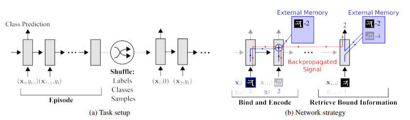
Also the training task setup, in each training episode the truth label is presented with a time offset label. i.e the actual label y_t  is presented with the one-step offset (x_t+1,y_t)

This prevents the neural network to simply map class labels to outputs, therefore the model has to memorize the information and the memory has to hold the information until the label information is presented later(t+1 in this case).

The controllers employed in our model are either LSTMs, or feed-forward networks. The controller interacts with an external memory module using read and write heads for the operation that are required on the external memory block

Reading from Memory:  Given some input x_t, the controller produces a key k_t, which is then used to fetch a particular memory from a row; i.e., M_t(i). During the read operation, the memory is addressed using cosine similarity which is used to produce a read-weight vector computed according to softmax.

Writing into memory: The mechanism for writing new information into memory operates a lot like the cache replacement policy. The Least Recently Used Access (LRUA) writer is designed for MANN which prefers to write new content to either the least used memory location (so that frequently used information is not lost) or the most recently used memory location(update the memory with newer and more relevant information).

Use Case: Multi Label Character Recognition on Omniglot Dataset

After training the MANN on 100,000 episodes with five randomly chosen classes with randomly chosen labels, the network was given a series of test episodes. In these episodes no learning happened and the network was to predict the class label of a never seen before class.

The performance of this classification was compared to human performance to check how efficient the MANN was.

The participants were shown an image and they were asked to choose an appropriate digit label. After the image disappeared the correct label was presented regardless whether the label predicted by the participants were correct or not allowing them to further reinforce correct decisions. After a short delay, a new image occurred and the prediction process was repeated and the participants were not allowed to view the previous images or use a pad as an external memory.

Surprisingly the performance of MANN surpassed that of humans on each instance, also the random guessing on the first instance was also better in MANN.

Performance Comparison:

MODEL	Instance(% correct)
	1st	2nd	3rd	4th	5th
Human	34.5	57.3	70.1	71.8	81.4
Feed Forward	24.4	19.6	21.1	19.9	22.8
LSTM	24.4	49.5	55.3	61	63.6
MANN	36.4	82.8	91	92.6	94.9

Source: One-shot Learning with Memory-Augmented Neural Networks

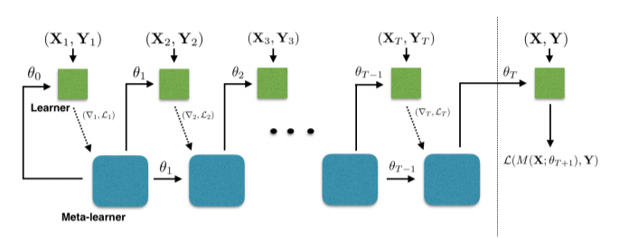
2. Optimization as a model for Few-Shot Learning :The aim here is to have an additional neural network for optimization of parameters. The meta learner here efficiently updates the learner’s parameters so that the learner can adapt to the new task quickly. Here the idea is to have 2 neural networks, one learner and the other meta learner. The meta learner model takes in loss and gradient of the parameters of the learner network and learns how to update the parameter

The update for learners parameter at time t with learning rate t

Θ_t = Θ_t−1 − α_t ∇_θt−1 L_t 

Below is an architecture diagram of how Meta-Learning can be used for optimization.

Experiment : 

For this experiment we have a learner which is a simple CNN with 4 layer Conv network; each with kernel size (3,3) and 32 filters, followed by batch normalization, ReLU non linearity and a (2,2) max pooling layer and having a final softmax layer for the number of classes considered

For the meta learner, we have a 2 layer LSTM where the first layer is a normal LSTM and the second one is a modified LSTN meta learner.The gradients and losses are fed into the first layer LSTM and the regular gradient coordinates are used by the second layer LSTM.

The data set used is a custom built Mini-Imagenet dataset by selecting a random 100 classes from ImageNet and picking 600 examples of each class and using 64, 16, and 20 classes for training, validation and testing, respectively. Considering 1shot and 5-shot classification for 5 classes. We use 15 examples per class for evaluation in each test set. 

The benchmark that are used to compare the performance are 

• Nearest neighbour baseline where the network is trained to classify between all the classes jointly in the original meta-training set. At metatest time, for each dataset D, we embed all the items in the training set using our trained network and then use nearest-neighbor matching among the embedded training examples to classify each test example
• Matching network which is a recent meta learning technique which has achieved state of the art results in few shot learning

Paper Source : Matching Networks for One Shot Learning

Model	5 class Classification(classification accuracy with 95% confidence)
	1-shot	5-shot
Nearest Neighbour Baseline	41.08	51.04
Matching network	43.40	51.09
Meta Learner LSTM	43.44	60.60

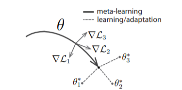
3. Model Agnostic Meta-Learning: This is an optimization algorithm that can be used with any algorithm that learns through gradient descent.

The basic idea of MAML is to find the better initial parameters so that with good initial parameters the model can learn quickly on new tasks with lesser gradient steps.

For example, let’s say we have a classification problem where we start by initializing random weights and minimize the loss using gradient descent. Gradient descent will find optimal weights that will give minimal loss by taking multiple gradient descent steps to find optimal loss and reach convergence.

In MAML we try to find these optimal weights by learning from the distribution of similar tasks so that we don’t have to start with randomly initialized weights instead, we can start with optimal weights which will take lesser gradient steps to reach convergence.

In the below diagram model-agnostic meta-learning algorithm (MAML), which optimizes for a representation θ that can quickly adapt to new tasks.

Experiment : Illustrative Regression Experiment

Objective is to see how quickly can the algorithm learn a new real valued function (sinusoidal function with varying amplitude and frequency ). 

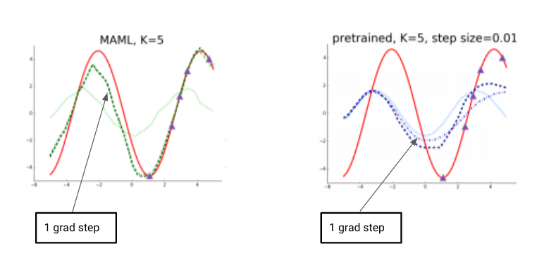
The red sine curve is an example curve that we are trying to learn and the purple dots are the 5 data points which will help in learning the function.

With just one gradient step and 5 data points MAML was able to learn very closely how to match the curve. It is interesting to see that though the data points are from the right side of the curve the algorithm is able to learn that this is a sinusoidal curve and has a high amplitude on the left as well. So it is safe to say that it is not just interpolating.

Other use cases for MAML would be 2D Navigation and Locomotion using Reinforcement learning. 

Conclusion

Meta-Learning is an exciting trend in the area of AI research as it will allow machines to make better decisions and also improve their decision-making by tuning their hyperparameters. Meta-learning is not limited only to semi-supervised tasks and can be used across multiple domains like recommendation systems etc. Meta-learning is a vast topic and this area has recently seen rapid growth in interest. Although there is some confusion about where this can be applied to and how it can be benchmarked but the scope of this in the near future is immense.