


A data analyst would frequently want to know whether there is a significant difference between two sets of data, usually pre- and post- campaign, and whether that difference is likely to occur due to random fluctuations or is instead unusual determining the existence of difference.
What is Matched-Pair Analysis?
MPA involves two groups: a study group and a comparison group, that are made by individually pairing study subjects with the comparison group subjects.
There are usually two situations in analyzing the related data:
- When we take repeated measurements from the same set of participants
- When we match item or participant according to some characteristic
In either situation, the analysis is conducted on the difference between two related values rather than individuals themselves. Since, the groups are comparable – the difference determines the statistically significant difference.
Why Matched-Pair Analysis?
The purpose of matched samples is to get better and accurate output in determining significant difference by controlling the effects of all other characteristics. Since each observation is paired, apart from the one characteristic that is being analysed, all other characteristics remain the same for both cases. For example, if we are analysing the impact of a campaign conducted by a company in the beauty industry, you can control for age-related shopping behaviour by matching respective participants. The pairs can be the same person, thing or the same group of observations.
Types of Matched-Pair Analysis:
- The McNemar test – uses consistency on paired nominal data.
- The paired sample t test – compares the means for the two groups to see if there is a statistical difference between the study and comparison group.
- The Wilcoxon signed rank test – this test compares mean ranks.
Example:
Let us consider an e-commerce retailer who wants to determine the impact of dollar value discount on the conversion rate campaign across all states in the US.
It is important to note that, as a rule of thumb, all parametric tests require sample sizes >=30. As the sample size increases, the statistical power increases.
H0 : µD = 0 (There is no difference in the mean conversion rate before and after the implementation of campaign)
HA : µD > 0 (There is a difference in the mean conversion rate before and after the implementation of campaign)
Since, the objective is to identify whether the campaign results in significantly better conversion rates or not – the alternate hypothesis is to prove the difference is greater than 0.
| States | Before | After | Difference |
| Massachusetts | 1.86% | 2.01% | 0.15% |
| Colorado | 1.83% | 2.01% | 0.17% |
| Maryland | 1.79% | 1.91% | 0.11% |
| California | 1.77% | 1.88% | 0.11% |
| Washington | 1.71% | 1.77% | 0.06% |
| Connecticut | 1.70% | 1.74% | 0.04% |
| Minnesota | 1.70% | 1.74% | 0.04% |
| Utah | 1.66% | 1.74% | 0.08% |
| Virginia | 1.66% | 1.73% | 0.07% |
| Delaware | 1.62% | 1.70% | 0.08% |
Representations of null and alternative hypotheses:
- H0 : µD = 0
- HA1 : µD ≠ 0 (two-tailed)
- HA2 : µD > 0 (upper-tailed)
- HA3 : µD < 0 (lower-tailed)
There are 4 important assumptions in performing a test as listed below:
- The dependant variable must be continuous
- Observations are independent
- The dependant variable must be normally distributed
- The dependant variable cannot have outliers
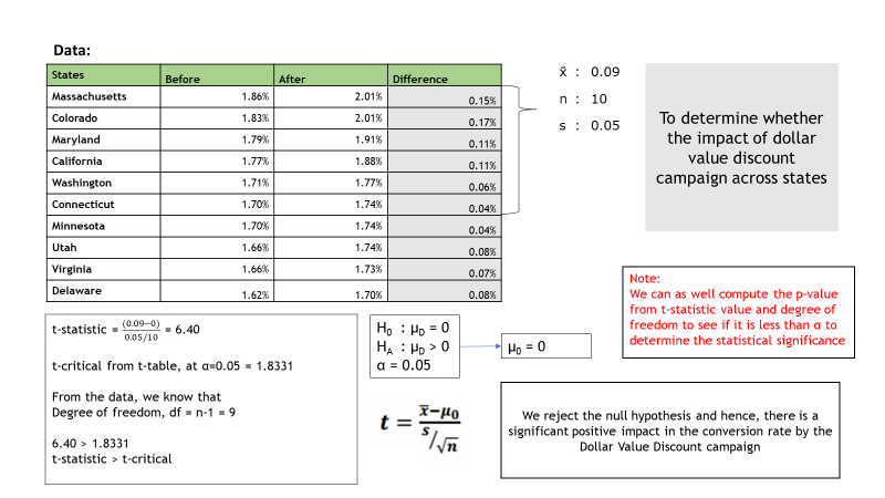
We reject the null hypothesis and state that the conversion rate is significantly better after the implementation of the campaign with 95% confidence (α=0.05) which means that the statistically significant difference in result is not by chance.