


Before going into causal analysis and inference at any depth, it is important to raise the following questions:
- How can we gauge change in consumer behaviour after we alter retail price of a product?
- How do you track the effectiveness of discounts in increasing sales?
- How can you monitor the success rate of your promotional emails?
The following aims to answer all those questions by first elaborating on the issues with traditional machine learning approaches.
REASON FOR EVOLUTION OF CAUSAL MODEL
For making decisions based on real-world data, we often go with a traditional machine learning model. The standard predictive machine learning model can identify the patterns in the data sets and predict accordingly, but the model does not explain the patterns or the reasons for their occurrence. It is not enough just to find statistical patterns in the data; the causal structure in the data also needs to be identified for making appropriate decisions.
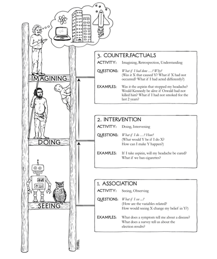
The above image is the ladder of causation stated in “The Book of Why” by Prof. Judea Pearl, who developed a theory of causal and counterfactual inference based on structural models. Most machine learning and complex deep learning models lie at the bottom-most rung of this ladder because they make predictions only based on associations or correlations amongst different variables. But they don’t give answers to the “what if? and why?” questions which are described in the 2nd and 3rd rung.
CAUSAL INFERENCE AND USE CASES
Causal inference refers to the process of drawing the conclusion that a specific treatment was the cause of the effect that was observed. The basic principle of causal analysis is to treat the cause rather than the symptoms. A root cause is a fundamental reason why something happens, and it can be quite distant from the original effect.
The Causal model helps to answer the following questions.
- What is the average treatment effect on the treatment outcome, and how does it work?
- Will treatment affect the individual unit positively or negatively?
- Is there any causal relationship between treatment and outcome?
- What is the effect of treatment on customers’ profit, and what treatment is recommended to them to invest in a multi-treatment scenario?
CAUSAL MODEL
For building causal models, we mainly use graph structures. However, it is important to understand certain causal terms before understanding a graph structure. Let us see about some essential terms like confounder, treatment, instrument, outcome, and treatment effect.
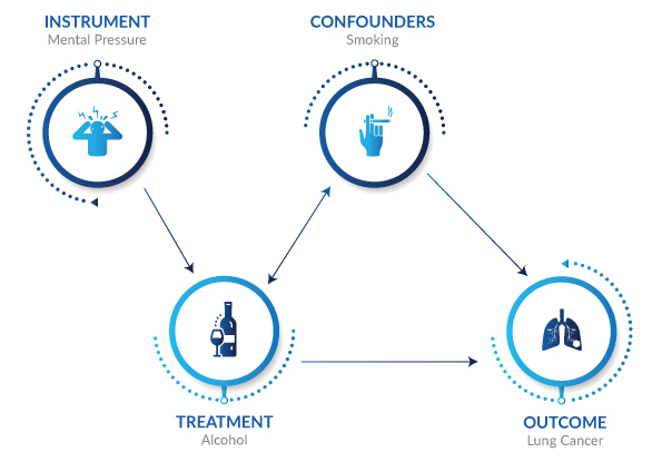
Confounders: A confounder (also confounding variable, confounding factor, extraneous determinant, or lurking variable) is a variable that influences both the dependent variable and independent variable, causing a spurious association. For example, in the above image, smoking can cause both alcohol consumption and lung cancer.
Treatment: The variable having a direct effect on the outcome feature is known as the treatment variable. For example, in the above image, alcohol consumption and lung cancer are directly related, i.e., treatment variable is the cause of the effect in the outcome variable.
Instrument: Instrument variable is the one that has direct causal effect on the treatment variable but not on the outcome variable. For example, mental pressure may trigger a person to drink alcohol, but it is not directly related to lung cancer.
Outcome: It is the one that depends or gets influenced by the input feature/independent feature. Simply, it is the one that all the treatment features can manifest. For example, lung cancer is the outcome variable in the above image.
Treatment effect: It is the impact created by the treatment variable on the outcome variable. It highlights the difference between potential outcomes when treated vs when not treated. Some of the treatment effect types are listed below.
- ATE – average treatment effect. It is the average difference between the potential outcome when treated vs when not treated. It gives the global treatment, i.e., it is calculated at a population level. When the effect is calculated only for the treatment group, it is known as ATT (Average treatment effect on treated). When it is calculated only for the control group, it is known as ATC (Average treatment effect on control).
- ITE – Individual treatment effect. It is calculated when the treatment effect is calculated at individual level. It tells whether the treatment affects the outcome of an individual unit positively or negatively.
- CATE – Conditional average treatment effect. It is calculated at the subgroup level. It is the average individual treatment effect of the subgroup. Customer segmentation is done based on CATE value. It is also known as the heterogeneous treatment effect.
CAUSAL MODEL IMPLEMENTATION METHODS
Here, we explore the methods for implementing causal models in a real-world scenario. Many methods are available for causal model implementation – some of them come up with basic concepts, and some use machine learning concepts. Here is a list of some methods that will help us to build a causal model.
- Matching
In this method, the parameters having similar values of covariant, i.e., propensity scores, are grouped, and their treatment differences between treated and untreated units are calculated for finding ATE, ATT etc., Propensity score is a single number that summarises all the unit’s covariance. This method is like a standard regression method.
- Stratification
In this method, the entire group is split into homogeneous subgroups. Within each subgroup, the treated group and the control group are similar under certain measurements over covariates, and the treatment effect within each subgroup is calculated. This is mainly used to adjust selection bias.
- Doubly robust learning
This method is used when the dataset has too many features for statistical approach, or its effects are not modelled properly. It is recommended to use when the treatment variable is categorical, and all the potential confounders are observed. It helps to estimate heterogeneous treatment effects and uses machine learning algorithms for basic prediction.
- Forest-based estimator
This method can also be used when the dataset has too many features. Using a flexible nonlinear approach helps to estimate heterogeneous treatment effects and confidence intervals.
- Meta learners
This method can be used if we have multiple responses.
In Meta learners, we have four different types of learners.
- T – learner
By calculating the response function, the T learner helps estimate the conditional expectations of the outcome separately for control and treatment groups, and their differences gives the heterogeneous treatment effect of the treatment variable on the outcome variable.
- S – learner
The S-Learner is like the T-Learner, except that when we estimate the outcome, we use all predictors without giving treatment variables a special role. The treatment indicator is included as a feature similar to all the other features without the indicator being given any special role.
- X – learner
This method is used when the dataset contains more control groups than treatment groups. It mainly uses information from the control group to estimate treatment effect. This method can also handle overfitting problems.
- Domain adaptation learner
It uses domain adaptation techniques to account for covariant shifts among treatment arms.
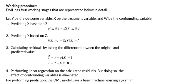
- Double Machine Learning (DML)
DML helps to estimate heterogeneous treatment effects and confidence intervals for measuring the uncertainty of the model. This method is recommended when we have a classification type of problem and for the one having a single response. The main advantage of this method is that it aims to correct both regularisation bias and overfitting bias by means of orthogonalization and cross fitting, respectively. DML also comes up with many variants like linearDML, sparseDML, causalforestDML, kernel DML, etc., and it will be used based on the type of dataset.
Use case of the application of a causal model to make decisions in the real-world scenario:
In this case, our main goal is to find the features that mainly influence credit card preference. It will be helpful for the client to do an effective campaign by choosing the right method for a particular customer with minimal cost.
The dataset was obtained from a multinational hospitality company. The obtained dataset contains 297 attributes which includes demographic information, stay details, services details and so on.
For training the model, suitable attributes that contribute more towards the outcome are selected based on domain knowledge. For example, to find the treatment/causal effect of ‘campaign variable’, all the related features need to be fetched from the similar period. Hence for model implementation, only features collected for a one-month duration are considered for training the causal model.
Traditional machine learning model
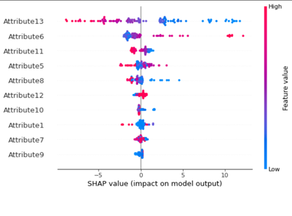
We first build a model based on a traditional machine learning approach by using light gradient boosting. By using Shapley value, the feature having a high impact on the outcome is ordered.
The results obtained from traditional ML are tabulated below
| Overall accuracy for train data | 0.89 |
| Overall accuracy for test data | 0.94 |
| % of predicted positive response | 0.83 |
| % of predictive negative response | 0.95 |
Drawbacks
By observing, the traditional model mainly focuses on avoiding lost causes (predicting more accurate negative responses). But as per business perspective, models need to target the sample having a positive response (persuadable customer). Moreover, the traditional model doesn’t show whether the features have a positive impact on the outcome, the percentage of the feature’s influence and how the treatment on different features impacts different segments of the population.
Causal model
To understand the causal effect, we have moved from the traditional model to a causal model. For implementing the causal model, we choose double machine learning because our target variable is categorical, and we need only one response. The causal model helps to find answers to various causal questions like the following.
- What is the effect of treatment on the outcome globally and individually?
- Who are all the top customers we need to target for credit card purchases?
- Which segments of people respond negatively towards a particular type of treatment?
- Which customers need to be targeted for a particular type of treatment?
Firstly, defining and training the causal model is done with treatment, confounders, and outcome variables. From the causal model, we can get many causal results like,
For finding the global treatment effect, the features are sorted based on the p-value, which has above 95% of confidence based on ATE calculated on the entire population for top features.
| Feature | Point | Stderr | Zstat | P_value | Ci_lower | Ci_upper |
| Attribute13(Services) | 2.47E-01 | 8.28E-03 | 29.8 | 7.65E-195 | 2.30E-01 | 6.70E-01 |
| Attribute5(Room count) | 2.21E-01 | 1.15E-02 | 19.2 | 1.57E-82 | 1.98E-02 | 2.40E-02 |
| Attribute6(Campaigns) | 8.13E-04 | 5.37E-05 | 15.1 | 9.78E-52 | 7.07E-04 | 9.18E-04 |
| Attribute11(Nature of stay) | 4.61E-02 | 4.24E-03 | 11 | 6.41E-11 | 3.81E-02 | 5.47E-02 |
| Attribute8(Partnerships) | 5.41E-03 | 6.18E-03 | 6.54 | 6.04E-11 | 3.78E-02 | 7.03E-02 |
| Attribute10(Campaigns) | 3.85E-02 | 7.35E-03 | 6.23 | 4.77E-10 | 3.22E-02 | 5.06E-02 |
| Attribute1(Reviews) | 4.46E-02 | 9.01E-06 | 6.07 | 1.29E-09 | 3.39E-05 | 6.92E-05 |
| Attribute12(Length of stay) | 5.16E-05 | 5.80E-05 | 5.72 | 1.03E-08 | -4.44E-03 | -2.16E-03 |
| Attribute7(Campaigns) | -3.31E+00 | 3.87E-05 | -5.7 | 6.32E-07 | 1.17E-04 | 2.69E-04 |
| Attribute9(Guest count) | 1.49E-04 | 8.00E-05 | 4.98 | 5.72E-07 | -5.53E-03 | -2.39E-03 |
From the table above, it is clear that attribute 13, attribute 5 and attribute 6 which is basically a treatment variable features have a positive impact on the purchase of credit cards. However, Attributes like 7 (treatment variable), 12, 9 have a negative impact on the outcome. Thus, if more campaigns are done with attribute 7, less would be the choice for credit card purchases.
To predict the customer who is likely to purchase a credit card, customers are sorted based on the most influential causal features. Then we observed that for the top 20% of customers ranked by the causal model, almost 81% of customers showed interest in buying a credit card. It will be useful to target the right customer.
For each customer, corresponding regression coefficient of the treatment variable (marginal cost) obtained from CATE is be taken as a treatment cost, and they are segmented based on their response towards increase or decrease in treatment. For example, segmenting customers based on their response, when they receive an increased number of hotel mails. The impact of the hotel mails on the customer globally and individually is given in the below table.
| Customer Count | Population Percentage | Actual Positive response on latest campaign | Response percentage without/ with treatment | |
| Total | 20367 | 100% | 1960 | 9.60% |
| Predicted Negative effect | 20192 | 99% | 1786 | 9% |
| Predicted Positive effect | 175 | 1% | 174 | 99% |
The result shows that, for any campaign through hotel mails, we can focus only on 1% of customers to get 99% response, instead of 9.6% response on the entire population. This will help the company to target the right customer.
Hence, we can draw the inference that the causal model helps us to obtain multiple causal results, and that these results will be helpful in making accurate decisions under different circumstances.