A complete guide to Marketing Mix Modeling

The singular aim driving all marketing initiatives is to maximise the ROI on the production, sales and distribution of a certain product or service. Effective marketing can therefore be defined as having the right product at the right time at the right place and available at the right price. The concept of a marketing mix strategy, was first proposed in 1960 by marketing expert Edmund Jerome McCarthy. The marketing mix elements can be broken down into:

Product

A product can be either a tangible product or an intangible service that meets a specific customer need or demand.

Price

Price is the actual amount the customer is expected to pay for the product.

Promotion

Promotion includes marketing communication strategies like advertising, offers, public relations, etc.

Place

Place refers to where a company sells their product and how it delivers the product to the market.

The importance of developing a marketing mix lies in the fact that the success or failure of a product or service in the market can also be traced back to how accurate and efficient its marketing mix was. Here is a complete guide to everything your company needs to know about the importance of creating a marketing mix and how to develop a winning marketing mix strategy for your product in 2020.

What is Marketing Mix Modeling?

An accurate marketing mix model can be the difference between the success or failure of a product!

Marketing Mix Modeling definition

The key purpose of a Marketing Mix Model is to understand how various marketing activities are driving the business metrics of a product. It is used as a decision-making tool by brands to estimate the effectiveness of various marketing initiatives in increasing Return on Investment (RoI).

How does a Marketing Mix Model work?

Marketing Mix modeling breaks down business metrics to differentiate between contributions from marketing and promotional activities (incremental drivers) vs. other (base) drivers. These factors affecting marketing mix can be defined as:

Incremental drivers: Business outcomes generated by marketing activities like TV and print ads, digital spends, price discounts, promotions, social outreach, etc.

Base drivers: Base outcome is achieved without any advertisements. It is due to brand equity built over the years. Base outcomes are usually fixed unless there are any economic or environmental changes.

Other drivers: They are a sub-component of baseline factors and are measured as the brand value accumulated over a certain time period due to long-term impact of marketing activities.
Importance of Marketing Mix Modeling

Marketing Mix modeling offers several important benefits for marketers:

Impact of variables on marketing mix models

Developing an accurate forecast for sales is only possible by taking into account these main variables.

Marketing mix elements are broken down into three variables: incremental, base and other. These three categories are further subdivided into a range of factors that can influence the market performance of a product or service. Understanding each of these variables is crucial for marketers to make an accurate forecast of the effects of promotional activities and product distribution.

Base variables

The baseline is any impact achieved independent of marketing mix variables. They are influenced by various factors like brand value, seasonality and other non-marketing factors like GDP, growth rate, consumer sentiment, etc. Determining the baseline outcomes is critical to understand the impact marketing activities are having on a product’s performance and a product’s distribution.

Some of the base variables include:

1. Price: The price is a very significant factor in determining the other elements of the marketing mix strategy. Price determines the target consumer group as well as the strategy for advertising, promotion and distribution.

The pricing model is one of the key factors affecting marketing mix because:

Pricing communicates the value of the product to the customers and can have direct impact on business performance
Impact on pricing depends on the elasticity of the product

2. Distribution: In Marketing Mix Modeling, distribution refers to the number of stores or locations where the product is available, number of stock keeping units (assortment) and shelf life (velocity). The distribution strategy is influenced by the market structure, the firm’s’ objectives, its resources and of course, its overall marketing strategy.

Distribution of a product is key because:

Strong product distribution chain coupled with targeted marketing activities directly results in effective business outcome.
Strong assortment for a product enables consumers to have multiple options to actively research and purchase.

3. Seasonality: Seasonality refers to variations that occur in a periodic manner. Seasonal opportunities are enormous, and often they are the most commercially critical times of the year. For example, major share of electronics sales are around the holiday season.

Read our blog and infographic on Holiday Shopping Analytics to understand the impact of seasonality on sales.

4. Macro-economic variables: Macro-economic factors greatly influence businesses and hence, their marketing strategies. Understanding of macro factors like GDP, unemployment rate, purchase power, growth rate, inflation and consumer sentiment is very critical as these factors are not under the control of businesses but substantially impact them.

Incremental variables

All marketing mix elements can be broadly classified under three categories:

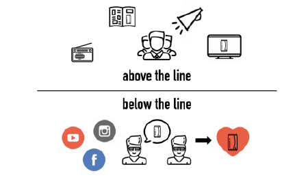
1. ATL (Above-the-Line) marketing: Above-the-line advertising consists of advertising activities that are largely non-targeted and have a wide reach. The primary objective of ATL activities is to help in brand building and to create consumer awareness and familiarity.

Examples of ATL marketing include television advertising, radio advertising, print advertisements (magazine and newspaper), and product placements (cinema and theatres).

Advantages of above-the-line marketing:

Tailored to reach a massive audience
Great for creating awareness
Long-term brand building

2. BTL (Below-the-Line) marketing: Below-the-line advertising consists of very specific, memorable and direct advertising activities focused on targeted groups of consumers. Often known as direct marketing strategies, below-the-line strategies focus more on conversions than on building the brand.

Examples of BTL activities include sales promotions, discounts, social media marketing, direct mail marketing campaigns, in-store marketing, events and conferences.

Advantages of below-the-line marketing

Specifically targeted towards individual customers
Drives immediate impact
Helps measure campaign effectiveness and conversions

3. TTL (Through-the-Line) marketing: Through-the-Line advertising involves the use of both ATL & BTL marketing strategies. The recent consumer trend in the market requires integration of both ATL & BTL strategies for better results.

Examples of TTL activities include 360° Marketing – campaigns developed with the vision of brand building as well as conversions and digital marketing (digital ads & videos).

Other variables

The long-term impact of several marketing initiatives can be grouped under:

1. Competition

Keeping a close eye on the competition is key to maintaining your brand’s edge.

Competition in the market can be either direct or indirect.

Direct competitors: Direct competitors are businesses that have the same product offerings. E.g. Apple iPhone acting as Competition to Samsung Galaxy
Indirect Competitors: Indirect competitors are those who don’t offer a similar product but meets the same need in an alternative way. E.g. Amazon Kindle and paperback books are indirect competition as they are substitutes

2. Halo and Cannibalization Impact

What is the halo effect?

Halo effect is a term for a consumer’s favouritism towards a product from a brand because of positive experiences they have had with other products from the same brand. Halo effect can be seen as a measure of a brand’s strength and brand loyalty. For example, consumers favour Apple iPad tablets based on the positive experience they had with Apple iPhones.

What is the cannibalization effect?

Cannibalization effect refers to the negative impact on a product from a brand because of the performance of other products from the same brand. This mostly occurs in cases when brands have multiple products in similar categories. For example, a consumer’s favouritism towards iPads can cannibalize MacBook sales.

In Marketing Mix Models, base variables or incremental variables of other products of the same brand are tested to understand the halo or cannibalizing impact on the business outcome of the product under consideration.

New variables emerging

With changing marketing environments, there are a number of new platforms emerging where brands are engaging actively with customers, especially millennial customers. This also leads to new marketing mix variables to be accounted for.

Some of these variables are

Product/Market Trend: Market trend/product trend is key in driving the baseline outcome of the product and understanding the consumer demand for the product.
Product Launches: Marketers invest carefully to position the new product into the market and plan marketing strategies to support the new launch.
Events & Conferences: Brands need to look for opportunities to build relationships with prospective customers and promote their product through periodic events and conferences.
Behavioural Metrics: Variables like touch points, online behaviour metrics and repurchase rate provide deeper insights into customers for businesses.
Social Metrics: Brand reach or recognition on social platforms like Twitter, Facebook, YouTube, blogs and forums can be measured through indicative metrics like followers, page views, comments, views, subscriptions and other social media data. Other social media data like the types of conversations and trends happening in your industry can be gathered through social listening.

Read our blog on Social Media Analytics and Monitoring to understand how new channels are impacting marketing for businesses.

Marketing Mix Methodology

Data preparation can help you identify key measurable metrics to that can impact your marketing mix model.

Each of the variable categories included when developing a strong marketing mix strategy involves a set of metrics that are used to measure the performance of different marketing activities

CATEGORY	VARIABLES	METRICS
BASELINE	BASE PRICE	Undiscounted price of the product at which it is sold in the market
	AVERAGE SALES PRICE	Discounted price at which the product is sold in the market
	ASSORTMENT (SKU)	Number of Stock Keeping Units of the product in a store/market to track the inventory of the product
	VELOCITY	Rate at which product is moving when it is available in store (Units/Store)
	DISTRIBUTION	Distribution of the product – No. of stores or No. of locations the product is available
PROMOTIONS	SALES PROMOTION	No of offers or No of days for which offers are running or the type of promotions like coupons, free shipping, price match guarantees, dollar-off etc.
DISCOUNTS	AVERAGE PRICE DISCOUNT	Average Price Discounts on the product at a particular time period
	WEIGHTED DISCOUNT	Average Price Discounts on the products weighted based on their share to product sales
SEASONALITY & HOLIDAY	SEASONALITY & HOLIDAY	Dummy variables to capture the spike/dip in KPIs during holidays like Thanksgiving, Christmas, New Year, Back to School, Labour Day, President Day, Retailer Promotions days like Prime Day etc.
MEDIA ACTIVITY	TV SPENDS	Marketing Spends for TV advertising
	REACH	Total No of consumers exposed to the ad
	FREQUENCY	Total No of times the customers are exposed to the ad
	TV GRP	Product of reach and frequency
	DIGITAL SPENDS	Marketing spends for digital advertising
	DIGITAL IMPRESSIONS	No of times the ads are exposed to customers
	DIGITAL CLICKS	No of clicks on online ads
	DIGITAL – OTHERS	Many other variables act as a measure for digital ads like click-through-rate, rich media, video view rate, cost-per-clicks, video likes, video comments etc.
	SEARCH SPENDS	Spends for Search marketing
	SEARCH IMPRESSIONS	Impression counted when Search page for product loads
	PRINT SPENDS	Marketing spends for product in a medium like magazines, newspapers etc.
	RADIO SPENDS	Marketing spends for radio advertising
COMPETITION	BASE	Base metrics for competition like pricing, distribution, seasonality, events, launches etc.
	MEDIA ACTIVITES	Competition media activities like spends, GRPs, impressions etc.
	OFFERS	Count of competition offers on different platforms
	DISCOUNTS	Discounts offered by competition on their products
OTHERS	SOCIAL MEDIA	Metrics to capture the activities of the brand or product on social media like page views, followers, sentiment score, reviews, likes, comment, retweets etc.
	EXTERNAL FACTORS	External variable affecting KPIs like macroeconomic factors
	TREND	The trend of product category or product over time period
	CYCLICITY	Metrics to capture product cycles like Sine or Cosine functions
	EVENTS & LAUNCHES	Indicative variables for capturing significant product launches, special events, conferences etc.

To learn more about the importance of data in marketing mix modeling, read our blog on Data-Driven Approach in Account-Based Marketing Campaigns.

In some cases, two specific instances can hamper marketers from developing a complete marketing mix model based on the above metrics:

Missing values
Outliers

Missing Value Treatment

What is a missing value?

One of the challenges in data analytics is missing values. A missing value is the non-availability of data for a particular observation or calculation in a variable. Usually, this happens because of errors during recording data or because of non-availability of data. Missing values may lead to biased variables, which in turn, may affect business outcomes.

Reasons for missing value

To resolve a missing value, we first need to understand why it occurred in the first place. Some of the most common reasons for a missing value are:

Data might not be available for the complete time period of analysis.
Non-occurrence of events.
People skipped response for some questions in surveys.
Non-applicability of questions in a survey.
Missing out in randomness.

Methods to treat missing values

Imputation: Imputation is a method where missing data is filled in with estimated values. Mean, median and mode are frequent imputation methods used.
Forecasting: Time series forecasting can be used to forecast/reverse-forecast the range of records that are not available. Apart from forecasting, we can use 4 weeks Moving Average to estimate missing values.
Replace with Zero: When data is available only if the transactions or a promotional event happened in a day, we should simply replace missing data with zeros to denote that there was no transaction or promotion for that day.
Deletion: A survey is the best example of an instance where deletion can fix missing values. In a survey, we cannot guess people’s choice and so it would be wise to delete rows with missing data.
Other: There are other sophisticated techniques for missing value treatment like prediction and KNN Imputation that can also be used if required.

Outliers

One of the key objectives of MMM is to try and explain the spikes, otherwise known as outliers. Outliers may or may not occur at random.
The reason for an outlier could be seasonality, a new product launch, campaign, promotion, discounts, competitor actions, etc. It could also be due to randomness. By differentiating outliers due to randomness from those caused by specific factors, you can include the right variables in the model and test them out to check if they explain outliers.
Example: Sales of electronics are much higher during product launches and holiday season like Christmas & Thanksgiving.

Read our blog on Marketing Mix Modeling: Challenges and Best Practices to learn more about how other common issues faced by marketers when developing a model can be resolved.

Types of Analysis in Marketing Mix Modeling

Through exploratory analysis, marketers can develop an understanding of the results of their marketing initiatives.

The statistical analysis involved in understanding the outcomes of various marketing activities can be broadly grouped into two different types:

Univariate analysis
Bivariate analysis

Univariate analysis

Univariate analysis is a form of quantitative evaluation where the data being analysed contains only one variable. Univariate analysis is primarily used to describe the data gained from marketing mix variables and find patterns that exist within them.

Patterns found in univariate analysis of a variable can be explained using:

Central tendency (mean, median & mode)
Dispersion (range & variance)
Maximum & minimum
Quartiles
Standard deviation

Univariate analysis is used to

Analyse the patterns in the data: E.g., Higher discounts are provided only during holiday periods

Identify the possibility of creating new variables: E.g., If there is a clear difference in discounts offered during the holiday periods and non-holiday periods, two separate discount variables could be created – holiday discounts and non-holiday discounts to test their impact

Identification of any outliers in the data – Univariate data can be visualized using

Frequency distribution tables
Bar charts
Histograms
Pie charts
Line charts

Bivariate analysis

Univariate analysis visualization

Line chart

TV Ratings	Frequency
1-50	20
51-100	17
101-150	21
151-200	7
201-250	1

Pie chart TV ratings

Bar chart

Histogram

Bivariate analysis is the analysis to understand the relationship between two different variables among marketing mix elements.

In MMM, Bivariate analysis helps us to

Identify the key variables that exhibit a good relationship with the dependent variable
Identify the type of relationship that the variable exhibits with the dependent variable

Types of bivariate analysis:

Numerical and numerical variables: Relationship between two numerical variables could be visualized using scatter plots and line charts.
Numerical and categorical variables: Relationship between numerical and categorical variables could be visualized using line charts or combination charts.
Categorical and categorical variables: Relationship between categorical and categorical variables can be visualized using stacked column chart and combination chart.

Data Transformation

Make the most accurate forecasts and efficient marketing mix models through data transformation.

Data transformation is the replacement of a variable by a function of that variable. For example, you can replace a variable X by the square root or logarithm of X.

The transformation, in essence, represents the response curve. Certain variables don’t have a linear relationship with sales. For example, TV GRPs usually have a nonlinear relationship with sales. Increase in TV GRP would increase the sales only to a certain extent, post which the growth would be saturated.

Bivariate analysis is the analysis to understand the relationship between two different variables among marketing mix elements.

There are generally two practical applications of data transformation:

Adstock effect
Lag effect

What is adstock effect?

Advertising adstock is a term used for measuring the memory effect carried over from the time of first starting advertisements. Marketers can use the advertising adstock as a variable in sales response modeling, such as regression analysis. It represents the half-life of advertisements.

What is lag effect?

A lag effect is used to represent the effect of a previous value of a lagged variable when there is some inherent ordering of the observations of this variable. This effect is useful in a study in which different subjects are given sequences of treatments and you want to investigate whether the treatment in the previous period is important to understand the outcome in the current period.

Understanding the adstock effect and lag effect are helpful in developing a marketing mix model to measure the impact of spending on advertisements. For instance, ads aired on TV might be remembered for longer than those on digital modes.

Significance of S-Curve transformations:

In reality, most of the advertising activities will have non-linear impact on the KPI’s and they exhibit a pattern of diminishing returns. Research has shown that initial advertising spends will have little impact until a certain threshold after which there will be a noticeable impact on the KPI’s can be observed. This impact tends to diminish as the spends reach a point of saturation post which there will be minimal impact. This entire impact can be captured in form of s-curve transformations. Gompertz, Chapman Richards and Weibull and Morgan-Mercer-Flodin transformations are typically better from a marketing mix perspective.

Marketing Mix Modeling Techniques

Wondering how you can build the most effective marketing mix model? These techniques can help you get started!

While the importance of a marketing mix is clear, most marketers are still unsure of how to build a marketing mix model. A technique known as ‘regression’ can predict the most efficient mix of all marketing variables. In regression, data is broken down into two categories: dependent variables (DV) and independent variables (IDV). The analysis of how independent variables can impact the outcome of dependent variables is the crux of regression. By doing this, marketers will be able to provide an accurate estimate of the marketing mix on the company’s net profits.

The most common marketing mix modeling regression techniques used are:

Linear regression
Multiplicative regression

1. Linear regression model

Linear regression can be applied when the DV is continuous and the relationship between the DV and IDVs is assumed to be linear.

The relationship can be defined using the equation:

Here ‘y’ is the dependent variable to be estimated, X are the independent variables and ε is the error term. βi’s are the regression coefficients. The difference between the observed outcome Y and the predicted outcome y is known as a prediction error. Regression analysis is mainly used for:

Causal analysis
Forecasting the impact of a change
Forecasting trends

However, this method does not perform well on large amounts of data as it is sensitive to outliers, multicollinearity and cross-correlation.

2. Multiplicative regression models

Additive models imply a constant absolute effect of each additional unit of explanatory variables. They are suitable only if businesses occur in more stable environments and are not affected by interaction among explanatory variables. But in scenarios such as when pricing is zero, the sales (DV) will become infinite.
To overcome the limitations inherent in linear models, multiplicative models are often preferred. These models offer a more realistic representation of reality than additive linear models do. In these models, IDVs are multiplied together instead of added.

There are two kinds of multiplicative models:

Semi-logarithmic models
Logarithmic models

Semi-logarithmic models

In Log-Linear models, the exponents of independent variables are multiplied.

Salest = exp(Intercept) * exp(β1*Pricingt) * exp(β2*Distributiont) * exp(β3*Mediat) * exp(β4*Discountst) * exp(β5*Seasonalityt) * exp(β6*Promotionst) *…

This can also be rewritten as

Salest = exp (Intercept + β1*Pricingt+ β2*Distributiont+ β3*Mediat+ β4*Discountst+ β5*Seasonalityt+ β6*Promotionst+ …)

Logarithmic transformation of the target variable linearizes the model form, which in turn can be estimated as an additive model. The dependent variable is logarithmic transformed; the only difference between additive model and semi-logarithmic model.

Ln (Salest) = Intercept + β1*Pricingt+ β2*Distributiont+ β3*Mediat+ β4*Discountst+ β5*Seasonalityt+ β6*Promotionst+ …

Some of the benefits of Log-Linear models are:

The coefficients β can be interpreted as % change in business outcome (sales) to unit change in the independent variables.
Each independent variable in the model works on top of what has been already achieved by other drivers. Hence, they are closer to real-time scenarios. A

Logarithmic Models

In Log-Log models, independent variables are also subjected to logarithmic transformation in addition to the target variable.

Salest = exp(Intercept) * β1*Pricingt * β2*Distributiont * exp(β3*Mediat) * exp(β4*Discountst) * exp(β5*Seasonalityt) * exp(β6*Promotionst) *…

Rewriting the model in linear form,

Ln (Salest) = Intercept + β1*Ln (Pricingt)+ β2*Ln (Distributiont)+ β3*Mediat+ β4*Discountst+ β5*Seasonalityt+ β6*Promotionst+ …

The main difference between Log-Linear and Log-Log models lies in the interpretation of response coefficients. In Log-Log models, the coefficients are interpreted as % change in business outcome (sales) in response to 1% change in independent variable

β = %ΔDependent_Variable / %ΔExplanatory_Variable

This implies constant elasticity of the target variable to explanatory variables. In Log-Linear models, elasticity cannot be directly estimated but can be calculated from the coefficient as β · X for every time period. It increases in absolute value with the explanatory variable.

Model Improvement techniques

Errors can impact the accuracy of your marketing mix model. Find out how these techniques can help you minimize errors in your model.

Invariably, errors often arise in marketing mix model predictions and actual outcomes. In many cases, a model might perform well on training data, but poorly on validation (test) data. To resolve this, marketers need to ensure there is a bias-variance trade-off.

What is a bias?

Bias is the difference between the average predictions of our model and the actual value we are trying to predict. Models with a high bias can lead to errors in training and test data.

What is variance?

Variance is an error which arises from sensitivity to small changes in the training set. Models with this error perform very well or training data, but have high error on test data.

Bias-variance trade-off

In a model, there are two common pitfalls that can occur. The model can have either underfitting (where the model is unable to capture underlying parameters) or have overfitting (where the model captures the noise along with the parameters). An underfitted model can have a high bias and low variance. On the other hand, an overfitted model can have low bias and high variance. Therefore, marketers need to strike a balance between the two with a bias-variance trade-off to develop an accurate model.

Regularization of data

To achieve this balance, regularization is an important tool. Through regularization, you can add a penalty term to the objective function and control the model complexity completely using that penalty term.

There are two main marketing mix modeling regression techniques for regularization are:

Lasso regression
Ridge regression
Elastic-net regression

Lasso regression

In lasso regression, we can minimise the objective function by adding a penalty term (sum of the absolute values of coefficients). This is also known as the least absolute deviations method. By penalizing the absolute values, the estimated coefficients shrink to zero such that overfitting is avoided and the learning is faster.

Ridge regression

In ridge regression, we try to minimize the objective function by adding a penalty term (sum of the squares of coefficients). When there is a multicollinearity problem among the predictor variables, the coefficient of one variable depends on other predictor variables included in the mode. By adding the penalty term, coefficients of collinear variables will shrink, except for the significant predictor among them.

Elastic-net regression

Elastic-net regression is a hybrid of ridge and lasso, combining the penalties of the two. This is usually the preferred method as it combines the best of both models.

Model Selection

Find out what goes into choosing the most appropriate model for your business.

Selection of the most appropriate marketing mix model is crucial for marketers to be able to make accurate predictions and estimations.
There are two main considerations to take into account when selecting a model:

Business logic

Market Mix Models have to be reflective of the actual market scenario. The model should be adaptive to changes in market over time.
For example, price of a smartphone could be elastic and so sales of this smartphone could be heavily dependent on pricing. If there is a significant increase in price, it might impact the sales of smartphone negatively. In such cases, product price can be used as a variable in the model to capture this trend.

From our extensive experience in developing marketing mix models, these are the key features that need to be implemented:

Media advertisements for the product should have positive coefficients in the model.
Halo or cannibalization can occur due to promotions for other products from the brand.
Halo impact from other products should be lower than the impact of marketing activities on the product.
Ad stock value for TVCs should be greater than for digital ads since TVCs have higher brand recall.
Discounts and promotions will have an immediate impact on sales
A product can be promoted by the brand who created the product as well as partners who sell that product.

You can also read our blog on Using Analytics to Cater to the Multi-Touchpoint Customer to help you build the most effective marketing mix model.

Statistical significance

Once the model has been generated, it should be checked for validity and prediction quality. Based on the nature of the problem, various model stats are used for evaluation purposes.
The following are the most common statistical measures in marketing mix modeling.

1. R-squared

R-squared is a statistical measure of how close the data are to the fitted regression line. It is also known as the coefficient of determination.
R-squared is always between 0 and 100%:
0% indicates that the model explains none of the variability of the response data around its mean.
100% indicates that the model explains all the variability of the response data around its mean.
General formula for R-squared is

Where SSE = Sum of squared errors and
SST = Total sum of squares

2. Adjusted R Squared:

The adjusted R-squared is a refined version of R-squared that has been penalised for the number of predictors in the model. It increases only if the new predictor improves the model. The adjusted R-squared can be used to compare the explanatory power of regression models that contain different numbers of predictors.

3. Coefficient:

Regression coefficients are estimates of the unknown population parameters and describe the relationship between a predictor variable and the response. In linear regression, coefficients are the values that multiply the predictor values.
The sign of each coefficient indicates the direction of the relationship between a predictor variable and the response variable.
A positive sign indicates that as the predictor variable increases, the response variable also increases.
A negative sign indicates that as the predictor variable increases, the response variable decreases.

4. Variable Inflation Factor

A variance inflation factor (VIF) detects multicollinearity in regression analysis. Multicollinearity is when there’s a correlation between predictors (i.e. independent variables) in a model. The VIF estimates how much the variance of a regression coefficient is inflated due to multicollinearity in the model. Every variable in the model would be regressed against all the other available variables to calculate the VIF. VIF is usually calculated as

Where Ri2 is R-squared value obtained by regressing “i”, the predictor variable against all other variables.

5. Mean Absolute Error (MAE)

MAE measures the average magnitude of the errors in a set of predictions. It’s the average over the absolute differences between prediction and actual observation where all individual differences have equal weight

Where yt is the actual value at time ‘t’ and
ŷt is the predicted value at time ‘t’

6. Mean Absolute Percentage Error (MAPE)

MAPE is the average absolute percent error for each observation or predicted values minus actuals divided by actuals:

Where yt is the actual value at time ‘t’ and
ŷt is the predicted value at time ‘t’

Quantification of Driver impact

Is your marketing mix model performing the way you intended it to? These techniques can help you calculate the success of your marketing mix model.

Once the model has been applied, marketers need to analyse the available data to judge the performance of the model.

There are two broad methods of analysis:

1. Contribution calculation

Business metrics are decomposed into base contributions and contributions due to seasonality and other factors. The marketing mix model helps identify key drivers of sales. Calculating contributions will depend on the type of model used:

Linear model

Assuming data is at weekly granularity,

From the MMM, we would get the regression equation (Business metric = Base + ®1* Driver1 + ®2*Driver2…)
where ® is corresponding coefficient for each driver
Predicted values are calculated at a weekly level (Predicted value = Base + ®1* Driver1 + ®2*Driver2…)
Multiply coefficient (®) with corresponding driver values at a weekly level to calculate driver contributions = ®1* Driver1, ®2*Driver2…

Log-linear model

Assuming data is at weekly granularity,

From the MMM, we would get the regression equation Ln (Business metric) = Base + ®1* Driver1 + ®2*Driver2…where ® is the corresponding coefficient for each driver
Predicted values are calculated at a weekly level (Predicted value = Base + ®1* Driver1 + ®2*Driver2…)
Multiply coefficient (®) with corresponding driver values at a weekly level to calculate driver contributions = ®1* Driver1, ®2*Driver2…

2. Due-to analysis

Due-to analysis explains the change in the contribution of each driver towards the business metric for different periods. With the help of due-to analysis, you can explain Year-On-Year (YOY) or Quarter on Quarter (QOQ) change in growth as a contribution to business metric from the drivers.

Read our blog on How to Measure Campaign Effectiveness Without a Control Group to understand how you can successfully attribute and measure campaign success.

Budget optimization

These factors are important in optimizing the budget for a marketing mix model.

Optimization is the process of arriving at most desirable solution from the list of all feasible solutions.
Optimization problems can be classified into different categories based on the type of constraints, nature of variables, nature of equations involved, permissible value of variables, number of objective functions etc.
There are multiple steps involved in designing a marketing mix optimization problem.

1. Constructing a model

This step involves specifying the model objective, model variables and model constraints for the problem.

Objective: This is a measure of the performance of the model that is to be minimized or maximized. For example, in the case of MMM, the objective function is generally to maximize KPI (Sales).
Variables: Variables are the components of the model that are to be optimized. For example, marketing drivers like TV Spends, Online Spends etc. are variables of the model.
Constraints: These are the functions that describe the relationships among the variables and that define the allowable values for the variables. For example, Total Spends for FY17 to be less than $100M.

2. Identifying algorithms for optimization

Once the model is constructed, suitable algorithms are chosen for optimization based on the nature of the optimization problem. There are numerous solvers available for optimization problems. Some of them (based on problem type) are:

Non-Linear Constrained Optimization: IPOPT, GRG Non-Linear, ANTIGONE, CONOPT, KNITRO, SNOPT etc.
Linear Optimization: BDMLP, Clp, Gurobi, OOQP, CPLEX etc.
Global Optimization: ASA, BARON, icos, PGAPack, scip etc.

3. Optimization solution

Results from optimization can be either global or local. This depends on the type of solving algorithms used. Hence for the same objective, different solvers return different types of solutions. The best possible solution is chosen based on the business context.

Global Optimal: This is the solution in which the optimization engine tries with all possible values of variables and ends up with one best solution for the objective.
Local Optimal: This is the solution in which the optimization engine has huge options for variables and upon solving, ends up with sub-optimal solution within a neighbouring set of solutions.

Read our blog on Data Analytics for CMOs : Using Digital Data for Consumer Insights

Scope for optimization

Marketing optimization is the process of improving marketing efforts to maximize desired business outcomes. Since the nature of MMM are mostly non-linear, non-linear constrained algorithms are used for optimization. Some of the use cases for marketing mix optimization are:

To improve current sales level by x%, what is the level of spends required in different marketing channels? E.g. To increase sales by 10%, how much to invest in TV ads or discounts or sales promotions?
What happens to the outcome metric (sales, revenue, etc.), if the current level of spends is increased by x%? E.g. On spending additional $20M on TV, how much more sales can be obtained? Where are these additional spends to be distributed?

You can also read our blog on How Conversion Rate Optimization Can Make or Break Your Sales to learn more about the importance of optimization in marketing mix modeling techniques.

These use cases answer the key areas for strategic planning like

Impact of Marketing levers
Optimization across different marketing channels
Optimization across time period

MMM – Optimization Case Study

We can understand the concept of marketing mix more effectively with a marketing mix modeling example. Consider a Product ABC from a leading retailer company. Marketing data for the product ABC is available for July to December 2017 (table below). With the available data, market mix models have been built with Sales as outcome (DV) variable and final marketing mix model equation is obtained.

Week	Sales	Pricing	Distribution	Competition Discounts	Competition Online Impressions	TV GRP	Online Impressions	Promotions	Discounts
07/01/2017	30,503	$1,067	48	1.12%	105.68 M	0	22.82 M	27	6.93%
07/08/2017	27,037	$1,068	47	4.33%	0.00 M	0	0.00 M	5	8.55%
07/15/2017	30,646	$1,038	42	1.89%	0.00 M	0	0.00 M	6	9.64%
07/22/2017	40,887	$954	35	1.10%	0.00 M	0	0.00 M	6	13.75%
07/29/2017	48,947	$912	31	4.56%	0.00 M	0	0.00 M	10	16.57%
08/05/2017	37,910	$1,010	38	3.64%	66.62 M	100	127.65 M	12	11.15%
08/12/2017	40,436	$1,007	37	1.66%	124.18 M	93	125.34 M	8	11.42%
08/19/2017	49,343	$994	33	2.50%	96.87 M	95	150.62 M	10	12.90%
08/26/2017	32,371	$1,078	39	5.08%	109.01 M	90	206.28 M	11	7.24%
09/02/2017	28,665	$1,060	40	1.10%	115.16 M	12	595.09 M	2	7.20%
09/09/2017	29,079	$1,061	42	0.00%	157.02 M	17	284.73 M	13	6.35%
09/16/2017	22,794	$1,098	41	0.15%	145.53 M	11	46.09 M	7	5.74%
09/23/2017	26,607	$1,048	36	0.02%	105.84 M	0	13.62 M	10	8.91%
09/30/2017	21,153	$1,100	39	0.00%	118.05 M	0	36.95 M	11	5.99%
10/07/2017	20,704	$1,092	42	0.00%	62.06 M	0	16.33 M	10	6.49%
10/14/2017	19,364	$1,082	44	2.10%	73.75 M	0	13.50 M	11	4.94%
10/21/2017	25,881	$1,050	53	3.13%	115.28 M	0	4.19 M	17	6.51%
10/28/2017	25,903	$1,018	46	2.30%	78.39 M	0	5.77 M	11	8.96%
11/04/2017	42,168	$996	54	1.08%	78.04 M	0	8.84 M	37	10.43%
11/11/2017	36,524	$1,002	57	7.11%	90.22 M	0	11.58 M	18	10.29%
11/18/2017	35,647	$1,014	55	7.44%	145.45 M	0	20.57 M	21	9.39%
11/25/2017	98,776	$948	41	16.57%	180.83 M	128	167.81 M	10	13.89%
12/02/2017	110,717	$935	52	5.62%	165.39 M	115	215.72 M	29	13.26%
12/09/2017	43,575	$1,039	56	0.00%	155.02 M	106	255.36 M	17	8.71%
12/16/2017	55,115	$1,000	52	5.19%	176.43 M	94	373.02 M	30	9.61%
12/23/2017	82,843	$961	40	4.87%	164.09 M	16	424.45 M	40	11.40%
12/30/2017	38,610	$1,072	53	2.07%	143.84 M	0	173.51 M	30	6.75%

Using weekly marketing data and market mix model equation, marketing optimization can be performed for various business cases.

Objective

What is the incremental lift in Sales (DV) when TV GRPs are increased by 20% from current level of 880 GRPs and discounts are increased by 10% from current level of 9.37%?

Procedure

The objective is to maximize the target variable (sales). Since TV GRPs and discounts are the variables to be optimized, constraints are applied to these variables.

Weekly maximum for TV GRPs will be decided by the sigmoid curve (based on saturation point). Total TV GRPs is set at 10% from current levels
Weekly maximum for discounts is set at value based on historic values. Average discounts is set at 20% from current levels

The following table lists the current levels and constraints levels for IDVs

Optimization Inputs	Actual Values	Target Values

Variable	Start Date	End Date	Minimum	Maximum	Value	Minimum	Maximum	Value
TV GRP	7/1/2016	12/30/2016	0	128	880	0	256	1052
Discounts	7/1/2016	12/30/2016	4.94%	16.57%	9.37%	0	20%	10.31%

These constraints are fed to the solvers and are optimized. Solvers provide optimized results for effective marketing plan

Result

The business recommendations, based on optimization results are as follows :

On increasing TV GRPs by 20% and Discounts by 10%, Sales increase of 21.90% is achieved upon effective distribution.
More TV GRPs are spent during holiday period (Nov-Dec) for effective sales
High levels of discounts are maintained during holiday period with no discounts in other period

The data summary for target variable and optimized variables are as follows

Output	Metrics	Minimum	Maximum	Average	Sum
	Actual	19,364	110,717	40,822	1,102,204
Sales (DV)	Optimized	15,733	148,732	49,761	1,343,554
	Lift %	-18.75%	34.33%	21.90%	21.90%
	Actual	4.94%	16.57%	9.37%	252.97%
Discounts	Optimized	0.00%	20.00%	10.31%	278.37%
	Lift %	-100%	20.68%	10%	10%
	Actual	0	128	32	880
TV GRP	Optimized	0	210	38	1052
	Lift %	0%	64.30%	20%	20%

The weekly distribution of target variable and optimized variables are shown in the below charts

You can read our blog on How Forecasting Is Changing Businesses Across Industries to learn more about the importance of developing a strong marketing mix model.

Conclusion

Marketing mix modeling techniques can minimize much of the risk associated with new product launches or expansions. Developing a comprehensive marketing mix model can be the key to sustainable long-term growth for a company. It will become a key driver for business strategy and can improve the profitability of a company’s marketing initiatives. While some companies develop models through their in-house marketing and analytics departments, many choose to collaborate with an external company to develop the most efficient model for their business.

Developers of marketing mix models need to have a complete understanding of the marketing environment they operate within and of the latest advanced market research techniques. Only through this will they be able to fully comprehend the complexities of the numerous marketing variables that need to be accounted for and calculated in a marketing mix model. While numerical and statistical expertise is undoubtedly crucial, an insightful understanding of market research and market environments is just as important to develop a holistic and accurate marketing mix model. With these techniques, you can get started on developing a watertight marketing mix model that can maximise performance and sales of a new product.

What is the definition of a marketing mix model?

A marketing mix model is the analysis of all the marketing activities considering the various metrics of product growth. It basically measures the success or failure of a product. The four important elements of marketing mix models are Product which can be a product or a service, Price that the customer pays, Promotion which are the marketing strategies that the firm undertakes and the Place where the product distribution takes place. Moreover, marketing models assess various marketing activities to check if these strategies have helped in increasing ROI.

What is an example of marketing mix?

Marketing mix is the process of analysing marketing initiatives and their corresponding outcomes. For example, consider a Product A which could be a product or a service that satisfies the customers’ needs. Next, look into the Price which is the amount that the customers would be paying for the particular product. Collect the marketing details for the product over a period of time, like the advertisements and forums which come under the category of Promotions. Also consider the Place where the product would be sold and how it is delivered to a particular place is important for building a model. Now, using the direct sales and few other factors, a marketing mix model is built.

What is marketing mix optimization?

Marketing mix optimization is the process of selecting a feasible solution after considering many possible solutions. The problems are categorized into different sections like nature of variables, equations involved, number of functions and many more. Analysing various factors classified into categories helps in finalising the solution after proper consideration.

How does marketing mix modeling work?

Marketing mix modeling analyses the product performance of a company. For this, there are a set of metrics allocated to evaluate the performance by drafting a model. The metrics could be the base price of the product, sales price, discount, average sales and many more. These set factors are together analysed and the model differentiates between marketing activities and other base factors to check the efficient functioning of the product in the product.

What is marketing mix modeling?

Marketing mix model is the process of checking the performance of a product. There are a few metrics like sales price, discount, average sales, etc. These values are assigned for coming up with an equation for the model. With the model data, marketing plans are reviewed and necessary changes are made if needed.

How to do marketing mix modeling?

Marketing mix models require the consideration of many factors like direct sales, Average sales, product promotion and discount to optimize the data. The data is collected for a particular period of time say, weekly or monthly. With the optimized marketing data, companies analyze their marketing strategies and refine their plans accordingly.

How to build a marketing mix model?

To build a marketing model, firstly, decide the objective of the model. The objective can be anything like increasing the sales. Next, fix the model variables like product spends, sales price, etc. These variables should be optimised. Later, finalise the model constraints that define the relationship of these variables. Then, identify the algorithms for optimization depending on the type of problem.

What are the limitations of marketing mix modeling?

There are a few limitations for the marketing mix model like obtaining accurate data is difficult and there is no particular standard to create the model. Moreover, this method is highly time consuming and also costly.

What is the difference between attribution and marketing mix modeling?

Marketing mix modeling is the statistical analysis of the performance of a product depending on the product’s marketing strategies whereas, attribution is a subset of the marketing mix model that analyzes the digital marketing channels.

Cookie	Duration	Description
cookielawinfo-checkbox-analytics	11 months	This cookie is set by GDPR Cookie Consent plugin. The cookie is used to store the user consent for the cookies in the category "Analytics".
cookielawinfo-checkbox-functional	11 months	The cookie is set by GDPR cookie consent to record the user consent for the cookies in the category "Functional".
cookielawinfo-checkbox-necessary	11 months	This cookie is set by GDPR Cookie Consent plugin. The cookies is used to store the user consent for the cookies in the category "Necessary".
cookielawinfo-checkbox-others	11 months	This cookie is set by GDPR Cookie Consent plugin. The cookie is used to store the user consent for the cookies in the category "Other.
cookielawinfo-checkbox-performance	11 months	This cookie is set by GDPR Cookie Consent plugin. The cookie is used to store the user consent for the cookies in the category "Performance".
viewed_cookie_policy	11 months	The cookie is set by the GDPR Cookie Consent plugin and is used to store whether or not user has consented to the use of cookies. It does not store any personal data.